이번 포스팅에서는
keras 에서 제공하는 mnist 데이터를 이용해
앞전 포스팅에서 학습한
CNN 모델을 생성해서 이미지 분류를 해보겠습니다.
1. mnist 데이터
mnist 는 손으로 쓴 글자를 모아둔
이미지 분류 datasets입니다.
mnist 데이터셋 분류는
CNN의 입문용, 모두가 거치는
"Hello world"
같은 단계라고하네요.
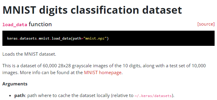
https://keras.io/api/datasets/mnist/#loaddata-function
Keras documentation: MNIST digits classification dataset
MNIST digits classification dataset [source] load_data function keras.datasets.mnist.load_data(path="mnist.npz") Loads the MNIST dataset. This is a dataset of 60,000 28x28 grayscale images of the 10 digits, along with a test set of 10,000 images. More info
keras.io
저는 keras의 dataset의
mnist digits classifiaction dataset를 이용해서 데이터를
받아오겠습니다.
이미지를 확인하고 싶은데
이미지의 정보는 나와있질 않습니다.
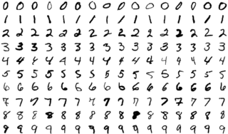
이미지출처 : https://en.wikipedia.org/wiki/MNIST_database
이런 형태의 이미지들입니다.
load_data() 함수를 사용하면 이미지 데이터를 받을 수 있습니다.
데이터 형태를 확인하고 가겠습니다.
x_train : (60000, 28, 28)
y_train : (60000,)
x_test : (10000, 28, 28)
y_test: (10000,)
튜블 형태의 train, test 묶음을 전달해주네요.

2. 데이터 가져오기
keras의 datasets 모듈의 mnist 를 import 해줍니다.
(numpy, pandas import 는국룰입니다.)
위의 문서에 나와있듯 load_data()를 통해
train, test의 두 튜플을 받아옵니다.
import numpy as np
import pandas as pd
from keras.datasets import mnist
(x_train, y_train), (x_test, y_test) = mnist.load_data()
받아온 데이터 형태가 위에서 확인했던 형태랑 같네요.
(이미지개수, 이미지폭, 이미지높, channel(RGB))
channel 1은 생략되었으니
훈련데이터만 보면
28x 28 의 흑백이미지 60000장이 입력값이네요.
출력값은 0~9까지의 10개의 클래스를 가진 데이터 60000개입니다.
print(x_train.shape , y_train.shape) #(60000, 28, 28) (60000,)
print(x_test.shape, y_test.shape) #(10000, 28, 28) (10000,)
unique, count =  np.unique(y_train, return_counts=True)
print(unique, count) #[0 1 2 3 4 5 6 7 8 9] [5923 6742 5958 6131 5842 5421 5918 6265 5851 5949]
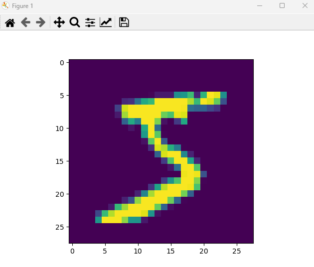
이미지 데이터는
matplotlib pyplot의 imShow()로 시각화해서
확인할 수 있습니다.
import matplotlib.pyplot as plt
plt.imshow(x_train[0])
plt.show()
3. 데이터 전처리
다중분류를 해주기 위해 출력값들을
Scikit learn OneHotEncoder()를 이용해
원핫인코딩을 해주겠습니다.
다중분류시 원핫을 하는 이유는 아래 포스팅을 참고해주세요.
https://aigaeddo.tistory.com/24
20. 분류2) 다중 분류 파헤치기(Multiclass Classification)
이번 포스팅은 이전 포스팅에 이어 다중분류(Multiclass Classification)에 대해서 파헤쳐보겠습니다. 해당 포스팅을 참고해서 학습하겠습니다. https://yhyun225.tistory.com/14 분류 (3) - 다중 분류(Multiclass Clas
aigaeddo.tistory.com
저는 원핫 처리시 Scikit learn의 OneHotEncoder()를
자주 사용해주는데 디코딩이 간편하기 때문입니다.
reshape를 해준 이유는 fit_trainform에는 행렬 형태만 들어가기 때문에
벡터를 행렬형태로 바꿔주었습니다.
x데이터는 conv2D 에 넣어주기 위해 reshape를 통해 행렬로 만들어주었습니다.
from sklearn.preprocessing import OneHotEncoder
ohe = OneHotEncoder(sparse=False)
y_train = ohe.fit_transform(y_train.reshape(-1,1))
y_test = ohe.transform(y_test.reshape(-1,1))

#conv2D는 4차원 행렬을 받음
x_train = x_train.reshape(x_train.shape[0], x_train.shape[1], x_train.shape[2], 1)
x_test = x_test.reshape(x_test.shape[0], x_test.shape[1], x_test.shape[2], 1)

unique, count =  np.unique(y_train, return_counts=True) #[0. 1.] [540000  60000]
print(unique, count)
이미지 데이터에 대한
스케일링 방식을 참고해서
255로 나눠 0~1사이의 값으로
만들어줬습니다.
#scaling
x_train = x_train/255
x_test = x_test/255
4. 모델구성

저는 위 이미지를 참고해서 모델을 구현할 예정입니다.
필요한 레이어들을 먼저 살펴보겠습니다.
Feature extraction 단
Layer는 keras의 layers 모듈에 있습니다.
Convolution Layer : Conv2D(),
Pooling Layer : MaxPooling2D()
(전 MaxPooling2D()를 사용하겠습니다.)
Classification 단
Flattenine Layer : Flatten(),
Fully Connected Layer : Dense()
코드로 구현해보겠습니다.
레이어들에 대한 사용법과 자세한 정보는
아래 keras 도큐먼트 페이지에서 확인하실 수 있습니다.
https://keras.io/api/layers/
Keras documentation: Keras layers API
Keras layers API Layers are the basic building blocks of neural networks in Keras. A layer consists of a tensor-in tensor-out computation function (the layer's call method) and some state, held in TensorFlow variables (the layer's weights). A Layer instanc
keras.io
Feature extraction 단 구성을 위해
위 그림처럼 Conv2D()레이어와 Padding()레이어를 2세트
모델에 넣어주겠습니다.
activation 함수에 relu를 설정해주었습니다.
(activation에 대해서는 따로 포스팅 하겠습니다!)
from keras.models import Sequential
from keras.layers import Dense, Flatten, Conv2D, MaxPooling2D

#Feature extraction
#Conv Layerset 1
model = Sequential()
model.add(Conv2D(64, (2,2), input_shape = (28,28,1), activation='relu'))
model.add(MaxPooling2D((2,2), strides=(2,2)))

#Conv Layerset 2
model.add(Conv2D(32, (2,2), activation='relu'))
model.add(MaxPooling2D((2,2), strides=(2,2)))
이후 Classification 단 구성을 위해
Flatten()레이어와 Dense()레이어를 넣어주겠습니다.
Output layer도 구성해줍니다.
Output 의 개수는 아까 데이터에서 확인한 클래스의 개수입니다.
마지막 레이어의 activation 함수는 다중분류이기 때문에 softmax입니다.
#Classification
#Flatten Layer
model.add(Flatten())
#Fully Connected Layer
model.add(Dense(256, activation='relu'))

#output layer
model.add(Dense(10, activation='softmax')) #class count : 10
3. 모델 컴파일 훈련
컴파일에서 다중 분류이기 때문에 loss 함수는 categorical_crossentropy,
optimizer 는 'adam'
metrics를 설정해서 acc를 체크하겠습니다.
모델 훈련은 일단 에폭5 , 배치 200, 발리데이션 0.2로 설정해주었습니다.
모든게 하이퍼파라미터이기 때문에 자유롭게 구성하시면 됩니다.
model.compile(loss='categorical_crossentropy', optimizer='adam', metrics=['acc'])
model.fit(x_train, y_train, epochs=5, batch_size=200, validation_split=0.2)
4. 평가 및 및 예측
모델이 완성되었으면
평가 및 예측값 확인을 해주시면 됩니다!
predict = ohe.inverse_transform(model.predict(x_test))
print(predict)
이번 포스팅에서는 CNN을 코드로 직접 구현해봤습니다.
이미지 데이터를 다루니까
데이터가 확실히 무겁네요!
이 이미지 데이터를 다루기 위해 앞선 포스팅에서
gpu로 돌리는 세팅을 했습니다.
더 큰 데이터를 다룰 그날이 오기를 바라며
계속 정진하겠습니다.
틀린점이 있다면 지적해주세요!
'인공지능 개발하기 > Machine Learning' 카테고리의 다른 글
| [Tensorflow] 28. ImageDataGenerator 이미지 데이터 증강(augument) (0) | 2024.01.27 |
|---|---|
| [Tensorflow] 27. ImageDataGenerator 이미지 데이터 전처리(preprocessing) (0) | 2024.01.27 |
| [Tensorflow] 25. CNN(Convolutional neural network) (0) | 2024.01.22 |
| [Tensorflow] 24. tensorflow GPU 가상환경 설정하기 (0) | 2024.01.20 |
| [Tensorflow] 23. 모델(Model) 구조와 가중치(Weights) 저장하기, 불러오기 (0) | 2024.01.20 |


